One way to see an elliptic curve is to view it as a smooth bidegree (2,2) curve in $\mathbb{P}^1\times\mathbb{P}^1$. This fact itself comes from the adjunction formula, but we suggest a way to derive a bidegree (2,2) formula from the Weierstrass equation. Based on that, we see how this connects with the tropicalized actions of Vieta involutions on elliptic curves.

Note on the Setup

All fields below are algebraically closed and has characteristic 0. This enables use to prove algebro-geometric claims by just looking at complex numbers (thanks to the completeness of the theory of algebraically closed fields of characteristic 0).

Bidegree (2,2) curves in $\mathbb{P}^1\times\mathbb{P}^1$

A simple computation using adjunction formula reveals that any smooth bidegree (2,2) curve X in $\mathbb{P}^1\times\mathbb{P}^1$ has trivial canonical bundle. That is, if we write $H_1,H_2$ for divisors of $\mathbb{P}^1\times\mathbb{P}^1$ given as $\ast\times\mathbb{P}^1$ and $\mathbb{P}^1\times\ast$ respectively (here $\ast$ is meant to be any point in $\mathbb{P}^1$), then the canonical bundle of X is computed as

So $H^0(X,K_X)=H^0(X,\mathcal{O}_X)=1=g$ tells that X has genus 1, i.e., is an elliptic curve.

One problem is that, it is hard to find a bidegree (2,2) curve which is smooth by just looking at cheap guesses. For instance, consider $\phi=0$ where

and $x,x’$ are respectively affine coordinates of the first and second factor of $\mathbb{P}^1\times\mathbb{P}^1$. In that case, if we flip the coordinates to $y=1/x$ and $y’=1/x’$ and consider

then this curve is singular at $(y,y’)=0$. So to avoid such a tragedy, we need to add $x^2x’,x(x’)^2,(xx’)^2$ terms into the polynomial $\phi$, making the verification that “$\phi=0$ is smooth” more complicated. Say, who would be happy to tune the parameters $a_{ij}$, $0\leq i,j\leq 2$ (from the scratch) such that

derives a contradiction?

Weierstrass Form, Weierstrass ℘

It is also known that any elliptic curve X can be embedded into $\mathbb{P}^2$, whose image is the curve with the equation, called Weierstrass form,

on the affine chart $[x:y:1]\in\mathbb{P}^2$. We also recall the group structure on elliptic curves, which is based on sketching lines between points in X. Checking this is quite standard (see, e.g., Silverman 2008 Sec. III.3), but the fact has more complex analytic significance.

It is also known that, if an elliptic curve is defined over $\mathbb{C}$, its complex points form a torus (see, e.g., Silverman 2008 Sec. VI.1) of complex dimension 1. So if we let $\Lambda\subset\mathbb{C}$ to be a lattice (a discrete copy of $\mathbb{Z}^2$) then $\mathbb{C}/\Lambda$ describes the complex points of an elliptic curve. Not only that, we have the Weierstrass ℘-function

which satisfies

where $G_4,G_6$ are Eisenstein series on the lattice (treat them as some special functions of $\Lambda$). It is known that the map

is injective and its image is precisely the curve $(y^2=4x^3-60G_4x-140G_6)\subset\mathbb{P}^2$. For sake of distinguishing, we name the map

and its image curve as

Any careful reader may notice that $i(0)$ is not well-defined just by what was written above. To get over this, we use that $\wp(z)=z^{-2}+O(z^{-1})$ and $\wp’(z)=-2z^{-3}+O(z^{-2})$, so that

\[[\wp:\wp':1]=[z^{-2}+O(z^{-1}):-2z^{-3}+O(z^{-2}):1] \\ =[z+O(z^2):-2+O(z):z^3]\]

near $z=0$. Plugging in 0, we then have $i(0)=[0:-2:0]=[0:1:0]$.

One nice aspect of this embedding is that it respects the group law on the elliptic curve. More precisely,

• three points $P,Q,R\in E(\mathbb{C})$ form an intersection of a line with $E$ iff $P=i(z_1),Q=i(z_2),R=i(z_3)$ satisfies $z_1+z_2+z_3=0$, and
• $i(0)=[0:1:0]$.

Hence we have $i(z_1)\oplus i(z_2)=i(z_1+z_2)$, where ⊕ denotes the group operation on $E$.

A relevant interesting exercise is to verify the determinant

\[\begin{vmatrix} \wp(z_1) & \wp'(z_1) & 1 \\ \wp(z_2) & \wp'(z_2) & 1 \\ \wp(-z_1-z_2) & \wp'(-z_1-z_2) & 1 \end{vmatrix}=0,\]

which can be shown by fixing $z_2$ and computing the pole order with respect to $z_1$. Of course there is a proof of above facts using more elegant methods (see Silverman 2008 Prop. VI.3.6).

Geometric description of ℘

Note that Weierstrass ℘-function is, over complex numbers, a map from a torus $\mathbb{C}/\Lambda$ to a sphere $\mathbb{P}^1(\mathbb{C})$. Furthermore, the ℘-function is an even function, and that evenness is the only source of non-injectivity; i.e., one has a

Lemma 1. We have $\wp(z)=\wp(z’)$ iff either $z=z’$ or $z=-z’$.

(Proof) The ‘if’ part comes from evenness of ℘. For ‘only if,’ let $x_0=\wp(z)=\wp(z’)$ and $z\neq z’$. On $\mathbb{P}^2$, $i(z)$ and $i(z’)$ stay on the line $x=x_0$ which passes through the point $[0:1:0]=i(0)$. Therefore $z+z’+0=0$. $\square$

The proof is motivated by the observation that the function ℘ works as the “x-coordinate” of the elliptic curve (in its Weierstrass form), the following is clear from the sketch of Weierstrass form elliptic curves figure source-Wikipedia:

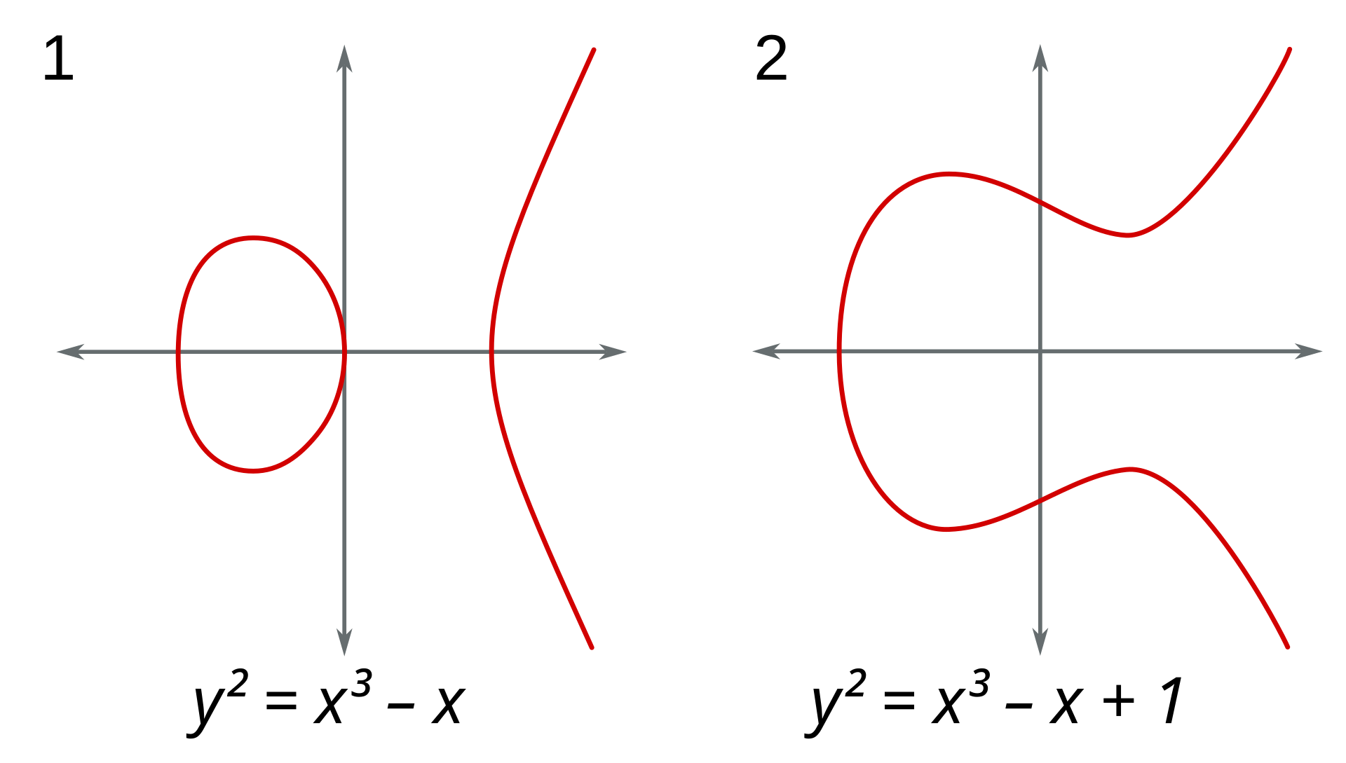
Having this observation on hand, one can geometrically describe the map of ℘ asthe natural quotient $\mathbb{C}/\Lambda\to(\mathbb{C}/\Lambda)/(z\sim-z)$ by antipodal points. The figure below describes a ‘pillowcase’ description of this quotient map.

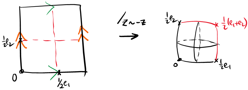
Another way to interpret this is to think ℘ as the quotient by a hyperelliptic involution. To describe the involution, we draw a line through a torus and rotate the torus by 180 degrees (hoping that we come back to the torus by doing so). If we identify points under this rotation then we form a sphere with four special points. figure source-Kashyap Rajeevsarathy

Now there is no reason to not consider other lines that can build hyperelliptic involutions, or their quotients. So consider $a\in\mathbb{C}/\Lambda$, and consider the function $z\mapsto\wp(z+a)$. Then $\wp(z)$ and $\wp(z+a)$ gives two hyperelliptic involutions on the torus:

For most choices of $a\in\mathbb{C}/\Lambda$, these involutions give an embedding of the torus into $\mathbb{P}^1\times\mathbb{P}^1$.

Proposition 2. Let $a\in\mathbb{C}/\Lambda$. Consider the map

\[\begin{array}{rl} \Phi_a\colon \mathbb{C}/\Lambda &\to (\mathbb{P}^1\times\mathbb{P}^1)(\mathbb{C}), \\ z &\mapsto(\wp(z),\wp(z+a)). \end{array}\]

This map injects iff $a\notin\frac12\Lambda/\Lambda$.

(Proof) We show the contrapositive. If $a\in\frac12\Lambda/\Lambda$, then $\Phi_a$ is an even map, which cannot be injective.

If $\Phi_a(z)=\Phi_a(z’)$ with $z\neq z’$, we have $z+z’=0$ and $(z+a)+(z’+a)=0$ by the above Lemma 1. But then $2a=0$, so $a\in\frac12\Lambda/\Lambda$. $\square$

From Weierstrass form to Bidegree (2,2) form

The Proposition 2 suggests an embedding of elliptic curves into $\mathbb{P}^1\times\mathbb{P}^1$ by hyperelliptic quotients. In fact this map can be described algebraically as follows. First, we fix a Weierstrass form

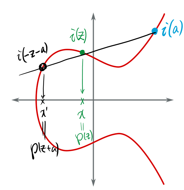
Fix a point $A=[\alpha:\beta:1]\in E$. For a point $P=[x:y:1]\in E$, define $Q=[x’:y’:1]\in E$ to be the third point so that $A,P,Q$ form an intersection of a line with $E$. Then define the map

Over the complex numbers, this coincides with the map $i\circ\Phi_{i^{-1}A}\circ i^{-1}$. Hence $\Psi$ is injective, as long as $2A\neq O$, or equivalently, $A\neq O$ and $\beta\neq 0$.

To study the image $\Psi(E)\subset\mathbb{P}^1\times\mathbb{P}^1$, we note that (see Silverman 2008 Algorithm III.2.3(d))

(There may be some issues regarding double points, but we ignore them for our computation now.) Note that, by collinearlity, we have

hence

Now we aim to get rid of $y,y’$ from \eqref{eqn:xx-formula}\eqref{eqn:x-formula}, to find a pure relation between $x,x’$. (We treat $\alpha,\beta$ as constants, as the point $A$ is fixed.)

Multiply $(\alpha-x)^2$ on both sides of \eqref{eqn:xx-formula}, and expand $(\beta-y)^2$. Then we have

If we replace $y^2=x^3+Ax+B$, then the cubic term $x^3$ are monic on both sides, letting us to cancel them out. Thus we have

Likewise, from \eqref{eqn:x-formula} we have

Hence

and squaring both sides we have

A bit of further algebra indicates that the relation \eqref{eqn:22-embedding} is defining a bidegree (2,2) curve in $\mathbb{P}^1\times\mathbb{P}^1$.

Proposition 3. The curve defined by the equation \eqref{eqn:22-embedding} is smooth and equals to the image curve $\Psi(E)\subset\mathbb{P}^1\times\mathbb{P}^1$.

(Proof) Call $C\subset\mathbb{P}^1\times\mathbb{P}^1$ for the curve defined by \eqref{eqn:22-embedding}. By the derivation, we have $\Psi(E)\subset C$.

Next, we claim that $\Psi$ is smooth and locally injective, which means for all point $P\in E$ we have $D_P\Psi\colon T_PE\to T_{\Psi(P)}\mathbb{P}^1\times\mathbb{P}^1$ injective. Recall the points $A=[\alpha:\beta:1]$, $P=[x:y:1]$ and $Q=[x’:y’:1]$. If one explicitly writes down $T_PE=\mathbb{C}.(2y\partial_x+(3x^2+A)\partial_y)$ and its image $(2y\partial_x+2y’\partial_{x’})\in T_{(x,x’)}\mathbb{P}^1\times\mathbb{P}^1$ (assume $P\neq O,-A$), then the required injectivity boils down to $y\neq 0\vee y’\neq 0$. This criterion, together with $2A\neq O$ for the injectivity when $P=O,-A$, forms a purely algebraic statement. Over complex numbers, this holds since $\Phi_{i^{-1}A}$ is smooth and (locally) injective, so is $\Psi$ over general fields.¹ Thus both $\Psi(E),C$ have dimensions 1, and furthermore $\Psi(E)$ is smooth (cf. Stacks Project, Lem. 29.34.19, with $S$ the Spec of the base field).

So it suffices to show that $C$ is irreducible. Note that the polynomial

over the polynomial ring of $x$ is irreducible iff $C$ is irreducible. This irreducibility is established if we have the discriminant

not a perfect square. One can check that $\Delta$ is a cubic polynomial, whose cubic term is $4\beta^2x^3$ (which is never zero since $2A\neq O$). So counting the degrees, we see that our discriminant is not a perfect square. $\square$

^{1. This argument is based on the model theory of algebraically closed fields of characteristic 0. If a statement is ‘purely algebraic,’ i.e., can be stated with constants from $\mathbb{C}$ and $+,-,\cdot$, its truth on $\mathbb{C}$ (which can be proven with whichever methods convenient) implies the truth on any algebraically closed field of characteristic 0. ↩}

Dynamics of Involutions

The bidegree (2,2) form \eqref{eqn:22-embedding},

is a quadratic equation in $x,x’$ if we fix $x’,x$ respectively. So there are natural algebraic involutions, Vieta involutions, that flip the two quadratic solutions. More concretely, one has maps

acting on $\Psi(E)\subset\mathbb{P}^1\times\mathbb{P}^1$ (cf. Proposition 3).

If we see this on complex numbers, the actions have a fairly nice visualizations. Note first that $s_x$ acts as the deck action on the 2-to-1 cover $x\colon E\to\mathbb{P}^1$ (note that $x$ is ℘ times some scale factor). Likewise, the 2-to-1 cover $x’\colon E\to\mathbb{P}^1$ has the deck action $s_{x’}$ (note that $x’$ is $\wp(z+a)$ times some scale factor).

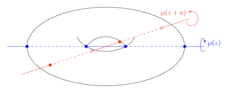
It turns out that both involutions $s_x,s_{x’}$ are hyperelliptic involutions. On the torus $\mathbb{C}/\Lambda$, we may express $s_x(z)=-z$ and $s_{x’}(z)=-2a-z$. These maps can be expressed by the figure below.

On the picture above, the axis with $\wp(z)$ passes the points in $\frac12\Lambda/\Lambda$, which are fixed under $s_x$. The axis with $\wp(z+a)$ passes the points in $-a+\frac12\Lambda/\Lambda$, which are fixed under $s_{x’}$. Now if we contract the meridian curve (more precisely, a simple closed curve transverse to the line $\mathbb{R}.(-a)$), we get two reflections on a circle.

If $a$ is a torsion element of order q≠2, then the orbit of a point by $s_x,s_{x’}$ forms a regular q-gon, and the involutions generate the dihedral group of the regular q-gon. Otherwise, we have an infinite dihedral group, which is the free product of order 2 groups $\langle s_x\rangle$ and $\langle s_{x’}\rangle$.

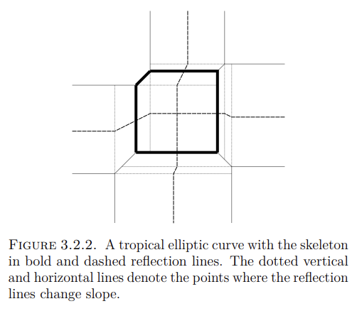
Such a ‘geometric simplificiation’ trick is captured by tropicalizations. If we tropicalize bidegree (2,2) curves like \eqref{eqn:22-embedding}, then we obtain a topological circle and Vieta involutions tropicalize to give reflections on that circle. Filip 2019, Figure 3.2.2, copied below, depicts such an idea.

Although the ‘geometric simplification’ discussed above looks like a coincidence due to the shape of tori, what was discussed in Filip 2019, Sec. 3 is somewhat opposite; it is the tropicalization that can systematically deal with such simplifications. In that regards, one can further study various algebraic actions in a geometric fashion, say as done in Spalding and Veselov 2020 and Filip 2019. Part of my thesis is based on the ideas of these previous works.

Update Log

• 230412: Created