This series of posts is aimed to be a rudiment of the Berkovich line, a locally compact space that “fills up” a non-archimedean field $K$. This post is the last of the series and continues from part 2.

Setups

We still use $(K,\vert\cdot\vert_K)$ for the fixed nonarchimedean, algebraically closed, and Cauchy complete field. We furthermore assume $K$ is non-discrete in the sense that there exists $x\in K$ with $\vert x\vert_K\neq 0,1$. Let $q>1$ be the number so that $\vert x\vert_K=q^{-v(x)}$ holds for all $x\in K$.

The following introduction to tropicalization comes from a text by G. Mikhalkin and J. Rau.

• Backlinks: tropical polynomial; Payne tropicalization

First Tropicalization: Amoeba

Consider the function

Suppose $p(z_1,\ldots,z_n)$ is a polynomial in $n$ variables. Then its (base $t$) amoeba $A_t(p)$ is defined as the $\mathrm{Log}_t$-image of the zero set of $p$. That is,

Example. Let $p(z_1,z_2)=z_1+z_2-1$. Then we sketch $A_t(p)$ as follows ($t>1$).

To see why we have this shape, for a point \((z_1,z_2)\in\{p=0\}\), put $u=\log_t\vert z_1\vert$ and $v=\log_t\vert z_2\vert$. Then from $1-z_1=z_2$, we have $\vert 1-t^ue^{\mathrm{i}\theta}\vert=\vert t^0-t^ue^{\mathrm{i}\theta}\vert=t^v$ for some $\theta\in\mathbb{R}$. So we see that $v$ is determined by a multivalued function

The sketch of the amoeba above is simply sketching this multivalued function. Furthermore, a more interesting shape occurs as $t\to\infty$.

If we continue with other $t$’s, and sending $t\to\infty$, we see that the amoebas $A_t(p)$ ‘converge’ to a shape. See (1) below.

This suggests to us that we have a ‘limit skeleton’ of the amoebas. See (2) above.

In general, as we send $t\to\infty$ (or $t\to 0+$), we can think of the ‘limiting amoeba’ $A_\infty(p)$ that vaguely sketches the shape of the amoeba $A_t(p)$ with $t>1$ big (or $t<1$ small).

Some algebra behind the scene

The ‘Amoeba’ Sum

Just like we introduced a multivalued function $u\oplus_t0$ above, we define

where \(\mathrm{Log}_t^{-1}x+\mathrm{Log}_t^{-1}y=\{z+w : \log_t\vert z\vert=x,\ \log_t\vert w\vert=y\}\). If we want to avoid this symbol, we may also define

Interestingly enough, if we take the limit $t\to\infty$, the interval above squeezes to a point (modulo some exceptions). Indeed,

Motivated by this, we define $x\oplus y:=\max(x,y)$, including the case $x=y$.

Similarly, one can define

but this is easily evaluated to $x\otimes_ty = x+y$, regardless of $0<t<\infty$.

Tropical Semiring

The limit operations $x\oplus y = \max(x,y)$ and $x\otimes y = x+y$ form an algebraic structure on \(\mathbb{R}\cup\{-\infty\}=[-\infty,\infty)\) called the (max-)tropical semiring. Indeed, the algebraic structure \((\mathbb{R}\cup\{-\infty\},\oplus,\otimes)\) satisfies the followings.

• \((\mathbb{R}\cup\{-\infty\},\oplus,-\infty)\) forms an abelian monoid¹
• \((\mathbb{R}\cup\{-\infty\},\otimes,0)\) forms an (abelian) monoid
• $-\infty\otimes x=-\infty$ for any $x<\infty$, and $x\otimes(y\oplus z)=(x\otimes y)\oplus(x\otimes z)$

This list is precisely the axioms of a (commutative) semiring.

Back to Amoeba

Now we make use of the algebra of $\oplus_t,\otimes_t$ to understand amoebas $A_t(p_t)$. For simplicity, we focus on the polynomials

where $a_j(t)$ are functions in $t$ that has the asymptotic growth

as $t\to\infty$. Note that this implies $\mathrm{Log}_ta_j(t) = c_j + o(1)$.

Call $(u,v)=\mathrm{Log}_t(z_1,z_2)$. Because $\mathrm{Log}_t(a_j(t)z_1^j) = (c_j +o(1))\otimes_t ju$, whenever $p(z_1,z_2)=0$ we have

That is,

If we take the limit $t\to\infty$ here, we fall into the following cases, depending on $u$.

1. If there is unique $j$ in which $(c_j\otimes ju)>(c_i\otimes iu)$ for all $i\neq j$, then $v=\mathrm{Log}_tz_2$ has the unique value according to $u=\mathrm{Log}_tz_1$.
2. If more than two $j$’s have the same $c_j\otimes ju$ values, then $v$ can be multivalued.

By this observation, by taking the limit $t\to\infty$ we get

for a finite set $S$. In that sense, we claim that the limit amoeba $A_\infty(p)$ is a graph of a function (to be called the tropicalization of $p_t(z)$) plus some vertical downward lines.

Remarks for $t\to 0+$

Another interesting algebra one can do is to consider the ‘amoeba’ sum when $t$ is small. Most of the notes above are still valid, with some fixes:

• $x\oplus_ty=[\log_t(t^x+t^y),\log_t\vert t^x-t^y\vert]\subset(-\infty,\infty]$,
• $\lim_{t\to 0+}x\otimes_ty$ is $=\min(x,y)$ when $x\neq y$, and $[x,\infty]$ when $x=y$.
• Setting $x\oplus y=\min(x,y)$ and $x\otimes y=x+y$, we have $(\mathbb{R}\cup{\infty},\oplus,\otimes)$ a (min-)tropical semiring.
• The numbers $c_j=\lim_{t\to 0+}\mathrm{Log}_ta_j(t)$ uses the limit $t\to 0+$ instead.
• The limit amoeba \(A_0(p)\subset\{v=\bigoplus_{j=0}^d(c_j\otimes ju) : u\notin S\}\cup\{v\geq\bigoplus_{j=0}^d(c_j\otimes ju) : u\in S\}\) sits on a graph plus some vertical lines upwards.

We see that, except for the max vs. min and $-\infty$ vs. $+\infty$, we observe that these two conventions are giving not much difference here.

However, for our purpose, we use the asymptotic $t\to 0+$ in the sequels. This is because this asymptotic has a better connection with the study of nonarchimedean fields. For instance, if we recall the Puiseux series, for the function \(a_j(t)\in\mathbb{C}\{\{t\}\}\), its growth degree $c_j=\lim_{t\to 0+}\mathrm{Log}_ta_j(t)$ can be evaluated as the valuation $c_j=v(a_j(t))$ (the least exponent that $a_j(t)$ has).

^{1. A set with an associative and commutative binary operator and an identity. So almost like a group but without inverses. ↩}

Tropical Polynomial

The above work introduces us the tropicalization of a polynomial $f_t(z_1)=\sum_{j=0}^da_j(t)z_1^j$, as

where \(c_j=\lim_{t\to 0+}\mathrm{Log}_ta_j(t)\)² is the growth degree. This definition naturally extends to multivariable polynomials, $p_t(z)=\sum_{j\in A}a_j(t)z_1^{j_1}\cdots z_n^{j_n}$,

So just like polynomials are sums of monomials, tropical polynomials are tropical sums of tropical monomials. Because each tropical monomial is an affine-linear function $w\mapsto c_j+j\cdot w$, we see that each tropical polynomial is a piecewise linear concave³ function.

Tropical Variety

Recall that \eqref{eqn:limit-amoeba} (or its $t\to 0+$ counterpart) tells that the polynomial $p_t=z_2-f_t(z_1)$ has the limit amoeba $A_0(p_t)$ mostly given as the graph of the tropicalization $\mathrm{trop}(f_t)(w_1)$. Some exceptions occur when two monomials in $\mathrm{trop}(f_t)(w_1)$ become the same.

But compare the ‘graph equation’ $w_2=\mathrm{trop}(f_t)(w_1)$ and the tropicalization of $p_t$, $\mathrm{trop}(p_t)(w_1,w_2)=w_2\oplus\mathrm{trop}(f_t)(w_1)$. The two look unrelated on the surface! Alas, there is still a way to relate them.

Proposition. (1) For a given $w_1\in\mathbb{R}$, suppose there is a unique $j$ such that $\mathrm{trop}(f_t)(w_1)=c_j+jw_1$. Then $w_2=\mathrm{trop}(f_t)(w_1)$ iff $w_2$ conicides with that minimal monomial $c_j+jw_1$.

(2) For a given $w_1\in\mathbb{R}$, suppose there are two $i\neq j$ such that $\mathrm{trop}(f_t)(w_1)=c_j+jw_1=c_i+iw_1$. Then $w_2\geq\mathrm{trop}(f_t)(w_1)$ iff $w_2\geq c_j+jw_1=c_i+iw_1$.

The proposition itself is trivial, but if we think $w_2=\mathrm{trop}(f_t)(w_1)$ or $w_2\geq\mathrm{trop}(f_t)(w_1)$ as a way to state $(w_1,w_2)\in A_0(p_t)$, the proposition boils down to the following

Corollary. We have $(w_1,w_2)\in A_0(p_t)$ iff two tropical monomials in $\mathrm{trop}(p_t)(w_1,w_2)=w_2\oplus\mathrm{trop}(f_t)(w_1)$ have the same value. Equivalently, the tropical polynomial $\mathrm{trop}(p_t)$ is not differentiable at $(w_1,w_2)$.

Motivated by this observation, we define the tropical variety of a tropical polynomial as follows.

Definition. A tropical variety of a tropical polynomial $\mathrm{trop}(p_t)(w)$ is the set of points $w\in\mathbb{R}^n$ where the tropical polynomial is not differentiable. Equivalently, it is the set of points $w$ where two or more tropical monomials of $\mathrm{trop}(p_t)$ coincide.

This notion answers the initial question: how do we find the limit amoeba $A_0(p_t)$? The answer is, find the tropical variety of $\mathrm{trop}(p_t)$!

Nonarchimedean tropicalization; the Fundamental Theorem

As remarked earlier, the growth degree of a Puiseux series is precisely the valuation of it: any function \(a(t)\in\mathbb{C}\{\{t\}\}\) has the formula $\lim_{t\to 0+}\mathrm{Log}_ta(t) = v(a(t))$. (The formula applies even for zero $a(t)\equiv 0$!) Thus it is natural to generalize the tropicalized polynomial for nonarchimedean contexts.

Suppose $K$ is as in the setup.

Definition. Let $f(x)\in K[x_1,\ldots,x_n]$, written as $f(x)=\sum_{j\in A}a_jx^j$. Define its tropicalization $\mathrm{trop}(f)(w)$ as

\[\mathrm{trop}(f)(w) = \min_{j\in A}(v(a_j) + j\cdot w).\]

Just as before, this defines a piecewise-linear concave function $\mathbb{R}^n\to\mathbb{R}$. The tropical variety thus generalizes also; but for this time, we generalize this for embedded affine varieties.

Definition. A tropical variety $V(\mathrm{trop}(f))$ of a tropical polynomial $\mathrm{trop}(f)(w)$ is the set of points \(w\in(\mathbb{R}\cup\{\infty\})^n\) where the more than two tropical monomials of $\mathrm{trop}(f)$ conicide.

Given an (embedded) affine variety $X\subset\mathbb{A}^n$ that intersects the torus \(T^n:=\{T\in\mathbb{A}^n : T_1T_2\cdots T_n\neq 0\}\), we define its tropical variety $\mathrm{trop}(X)$ by

\[\mathrm{trop}(X) := \bigcap_{f\in I(X)}V(\mathrm{trop}(f)),\]

where $I(X)\subset K[x_1,\ldots,x_n]$ is the ideal of polynomials vanishing at $X$.

Not only that, but the notion of ‘limit amoeba’ also generalizes, again for (embedded) affine varieties of $K$.

Notation. Suppose $X\subset\mathbb{A}^n$ is an (embedded) affine variety over $K$ that intersects the torus \(T^n:=\{T\in\mathbb{A}^n : T_1T_2\cdots T_n\neq 0\}\). Denote $\mathrm{Trop}(X)$ for a closed subset $\subset\mathbb{R}^n$ defined as

\[\mathrm{Trop}(X):= \overline{\{v(x)\in(\mathbb{R}\cup\{\infty\})^n : x\in X(K)\}}.\]

Here $x=(x_1,\ldots,x_n)$, and $v(x)=(v(x_1),\ldots,v(x_n))$.

Here is the nonarchimedean version of the ‘limit amoeba’ problem.

Fundamental Theorem of Tropical Algebraic Geometry (Diane and Sturmfels 2015, Thm 3.2.3). We have $\mathrm{trop}(X)=\mathrm{Trop}(X)$.

That is, the analytic problem, $\mathrm{Trop}(X)$, of finding the set of all possible valuations on a variety can be switched to a purely algebraic problem, $\mathrm{trop}(X)$, of finding ‘cracks’ of tropicalized polynomials.

Another significance of the theorem is this. If we think back the amoeba problem, when we defined the notion of tropical variety $\mathrm{trop}(X)$, we have used that two monomials $x,y$ sum to zero only if $v(x)=v(y)$, (complex case: $t^u+t^v=0$ only if $\vert t^u\vert=\vert t^v\vert$) so on each zero of a polynomial we have more than two tropical monoids coincide. So it is evident that each point $p\in X(K)$ has valuations $v(p)$ in the tropical variety $v(p)\in\mathrm{trop}(X)$. That is, $\mathrm{Trop}(X)\subset\mathrm{trop}(X)$.

But the other inclusion is not very obvious. Although $w\in\mathrm{trop}(X)$ morally tells we can have a point $p\in X(K)$ with valuations $v(p)=w$, finding an actual point $p$ is another task (in fact, approximations can be the best when $w\notin(K^\times)^n$). The theorem helps us to fill in such a gap, thus.

Newton Polygon; the Ball Norm

For $n=1$, tropicalizations are connected to more classical math on nonarchimedean fields, the Newton polygon. This concept does relate to Newton, for this is closely related to Newton’s method of finding solutions of polynomials with Puiseux coefficients (cf. a Mathoverflow answer). Once we know the growth degree (a.k.a. valuation) $c$ of a solution, then one can initiate the method with $x_0=\alpha t^c$!

Note. The use of Newton polygons is not particularly restricted to 1D. It is a useful tool for sketching $\mathrm{trop}(X)$ in higher dimensions.

Recall that a tropical polynomial $\mathrm{trop}(f)(w_1)$ is a concave, piecewise-linear function. There one can think of the Legendre transform of the convex function $-\mathrm{trop}(f)(-w_1)$.⁴ The convex function obtained in this way is called the Newton polygon.

Definition (Newton Polygon). Given a polynomial $f(x)=\sum_{j=0}^da_jx^j\in K[x]$ in one variable, we define its Newton polygon $NP_f(\lambda)$ by one of the following equivalent definitions.

1. The Legendre transform $NP_f(\lambda):=\sup_{w_1\in\mathbb{R}}\left(\lambda w_1 -(- \mathrm{trop}(f)(-w_1))\right)$ of the ‘tropicalized polynomial’
2. The greatest convex function $NP_f$ on $\mathbb{R}$ such that $NP_f(j)\leq v(a_j)$ for all $j=0,\ldots,d$

A more standard definition of the Newton polygon is given as the convex hull of the rays \(\{j\}\times[v(a_j),\infty)\subset\mathbb{R}^2\). However, this results in the epigraph \(\{y\geq NP_f(x)\}\) of a convex function $NP_f(x)$, so I call both the epigraph and the function as the Newton polygon.

The main use of this polygon is as follows.

Main Theorem of Newton Polygons (see B. Casselman’s note). The Newton polygon $NP_f$ is a piecewise linear convex function defined on a subinterval of $[0,d]$.^a List $\mu_1<\ldots<\mu_k$ for distinct slopes that $NP_f$ can have, and let $\lambda_1,\ldots,\lambda_k$ be the lengths of intervals where we have slopes $\mu_1,\ldots,\mu_k$ (respectively).

Then the original polynomial $f$ has $\lambda_i$ roots of valuations $-\mu_i$, for $i=1,\ldots,k$.

^{a. I am worried of the case when $a_0=0$ or $a_d=0$. If $a_0,a_d\neq 0$, then $NP_f$ is defined on $[0,d]$. ↩}

Corollary. For $f(x),g(x)\in K[x]$, we have $\mathrm{trop}(fg)=\mathrm{trop}(f)+\mathrm{trop}(g)$.

(Proof) It suffices to show that, for $f(x)=a\prod_{i=1}^d(x-\xi_i)$ with $\xi_i\neq 0$ for all $i$, we have $\mathrm{trop}(f)(w_1)=v(a) + \sum_{i=1}^d\min(w_1,v(\xi_i))$. Because $\mathrm{trop}(f)(\infty)=v(f(0))=v(a)+\sum_{i=1}^d\min(\infty,v(\xi_i))$, the problem reduces to comparing the derivatives. That is, we set our goal to show that

\begin{equation} \label{eqn:multiplicity-of-ball-norm} [\mathrm{trop}(f)]’(w_1) = \sum_{i=1}^d H(v(\xi_i)-w_1), \end{equation}

where $H(x)$ is the Heaviside function.

Align the roots $v(\xi_1)\geq\cdots\geq v(\xi_d)$ in decreasing valuations. Define $\varphi(w_1):=-\mathrm{trop}(f)(-w_1)$, and consider its Legendre dual $\varphi^\ast=NP_f$. By the main theorem, the derivative $NP_f’(\lambda)$ has values $-v(\xi_1)\leq\cdots\leq -v(\xi_d)$ at intervals $[0,1],[1,2],\ldots,[d-1,d]$ respectively. If we take the ‘inverse function’ of this, (a) we get the derivative $\varphi’(w_1)$, and (b) this $\varphi’(w_1)$ is a step function with $\varphi’(-\infty)=0$ and raises step 1 at $w_1=-v(\xi_i)$. In terms of the Heaviside function, this means

By the construction, we have $\varphi’(w_1)=[\mathrm{trop}(f)]’(-w_1)$. We have established \eqref{eqn:multiplicity-of-ball-norm}.

$\square$

Corollary. The ball norm $\vert\cdot\vert_{B(a,r)}$ on $K[T]$ is multiplicative.

(Proof) Write $f(T)=\sum_{j=0}^da_jT^j$. In the previous post we have shown that $\vert f(T)\vert_{B(a,r)}=\max(\vert a_j\vert_K r^j : 0\leq j\leq d)$. Taking $-\log_q$ on both sides,

It remains to use the formula $\mathrm{trop}(fg)=\mathrm{trop}(f)+\mathrm{trop}(g)$.

$\square$

This is the ‘proof that captures the complete sense that the theorem encodes,’ as remarked after the previous proof. The beauty lies in not just viewing $f(T)$ as an additive lump but turning it into a multiplicative lump to draw the multiplicativity as a natural result. Intermediate math was the Newton polygon, and I have devoted the first half of this post to introduce it.

<sup>2. To have an easier connection with nonarchimedean fields, from now on we use the ‘minimum’ convention. Hence $x\oplus y=\min(x,y)$ here. ↩
3. This is because our tropical sum is taking minima. For versions taking maxima, tropical polynomials are convex. ↩
4. Bit ugly, but this treatment was made to be more coherent with standard references. ↩</sup>

Berkovich Line is the Limit of Tropicalizations

The following theorem is the core reason why we have talked about tropicalizations.

Payne’s Tropicalization Theorem (Payne 2009, for Berkovich lines). Let $K$ be as in the setup. For each finite subset $I\subset K$, define the map $\pi_I\colon(\mathbb{A}^1_K)^{an}\to(-\infty,\infty]^I$ by

\[\pi_I(x):=\left(-\log_q\vert T-a_i\vert_x\right)_{a_i\in I},\]

and define the set \(\mathbf{Trop}(\mathbb{A}^1,I)=\overline{\{\left(v(x-a_i)\right)_{a_i\in I} : x\in\mathbb{A}^1(K)\}}\subset (-\infty,\infty]^I\). Then writing $\varprojlim\pi_I$ for the inverse limit of the maps $\pi_I\colon (\mathbb{A}^1_K)^{an}\to\mathbf{Trop}(\mathbb{A}^1,I)$, we have a homeomorphism

\[\varprojlim \pi_I\colon (\mathbb{A}^1_K)^{an}\xrightarrow{\sim}\varprojlim_{\substack{I\subset K \\ I\text{ finite}}}\mathbf{Trop}(\mathbb{A}^1,I).\]

Remark. The statement above is a simplified version of the original. The original statement takes inverse limits over all embeddings $\iota\colon\mathbb{A}^1\hookrightarrow\mathbb{A}^{m(\iota)}$, in the category of embeddings with morphisms being toral equivariant. There the statement considers the tropical set $\mathbf{Trop}(\mathbb{A}^1,\iota):=\mathrm{Trop}(\iota(\mathbb{A}^1))$ based on the embedded variety. With this careful setup the original statement is powerful enough to cover all affine varieties $X$ over $K$, not just $X=\mathbb{A}^1$.

Here my simplification lies in restricting the embeddings to linear ones $\iota_I\colon\mathbb{A}^1\hookrightarrow\mathbb{A}^{I}$, $T\mapsto\left(T-a_i\right)_{a_i\in I}$, so that I can avoid discussing toral equivalence and rather stick to the inclusions of the indices $I$. Such a decision does not lose the generality, as this subfamily is a cofinal family of Payne’s original. See appendix for the details.

Preparations

Recall that $A=K[T]$ is a unique factorization domain (UFD). If $K$ is algebraically closed, we can list all irreducible elements of $A$ as $(T-a)$, $a\in K$. Therefore we determine a point \(x\in(\mathbb{A}^1_K)^{an}\) by looking at the norm values \(\left(\vert T-a\vert_x\right)_{a\in K}\) of linear polynomials, or their logarithms \((-\log_q\vert T-a\vert_x)_{a\in K}\).

This data allows us to embed the line $(\mathbb{A}^1_K)^{an}$ into a smaller product space.

Compare this with the embedding \((\mathbb{A}^1_K)^{an}\hookrightarrow\prod_{f\in K[T]}[0,\infty)\cong\prod_{f\in K[T]}(-\infty,\infty]\) seen in a previous post/part 1. The product was held over all polynomials back then, and now we have reduced it to linear monic polynomials!

Nonetheless, we still have an infinite product space, so we need to work a bit to convince us that this embedding is worth taking a look at.

Finite Approximation Scheme

An idea here is, instead of looking at the infinite product space as a whole, we look through a finite sub-products. In case of the Berkovich line $(\mathbb{A}^1_K)^{an}$, it is done as follows.

For each finite subset $I\subset K$, denote the natural projection \(\pi_I\colon\prod_{a\in K}(-\infty,\infty]\twoheadrightarrow(-\infty,\infty]^I\). Write \(\pi_I\left((\mathbb{A}^1_K)^{an}\right)\) for the image of \(\pi_I\circ ev\colon(\mathbb{A}^1_K)^{an}\hookrightarrow\prod_{a\in K}(-\infty,\infty]\twoheadrightarrow(-\infty,\infty]^I\). Then we have a natural map

If the map $\varprojlim\pi_I$ is a surjection, then it is a homeomorphism; see the appendix. That is, we have $(\mathbb{A}^1_K)^{an}$ formed by ‘stacking up’ finite approximations $\pi_I\left((\mathbb{A}^1_K)^{an}\right)$ once we know the surjectivity.

Understanding Finite Approximates

Understanding $(\mathbb{A}^1_K)^{an}$ via \eqref{eqn:finite-approximation} means that we pass the problem to understanding $\pi_I\left((\mathbb{A}^1_K)^{an}\right)$, with $I\subset K$ finite. This will be done in three steps. (Here, $\mathbb{A}^1(K)\subset(\mathbb{A}^1_K)^{an}$ is the subset of evaluation norms.)

1. Understand what the closure $\overline{\pi_I(\mathbb{A}^1(K))}$ is, i.e., what is the closure of the set \(\{\left(v(x-a_i)\right)_{a_i\in I} : x\in K\}\subset(-\infty,\infty]^I\).
2. See if $\pi_I\left((\mathbb{A}^1_K)^{an}\right)=\overline{\pi_I(\mathbb{A}^1(K))}(=\mathbf{Trop}(\mathbb{A}^1,I))$.
3. Show that \(\varprojlim\pi_I\colon (\mathbb{A}^1_K)^{an}\to\varprojlim_{I\subset K}\pi_I((\mathbb{A}^1_K)^{an})\) is a surjection.

Step 1

This is a step where the fundamental theorem plays its role. Declare the embedding $\iota_I\colon\mathbb{A}^1\hookrightarrow\mathbb{A}^I$ by $T\mapsto(T-a_i)_{a_i\in I}$, and let $X_I=\iota_I(\mathbb{A}^1)$. Then the definition of $\mathbf{Trop}(\mathbb{A}^1,I)$ above is just $\mathrm{Trop}(X_I)$. Because $\overline{\pi_I(\mathbb{A}^1(K))}=:\mathbf{Trop}(\mathbb{A}^1,I)=\mathrm{Trop}(X_I)=\mathrm{trop}(X_I)$, we choose the object of study by our convenience.

Example 1. Suppose \(I=\{a,0\}\). Then $X_I\subset\mathbb{A}^2$ is given by an equation $T_2=T_1+a$. Hence $\mathrm{trop}(X_I)$ is given by the locus where the minimum in $f(w_1,w_2)=\min(w_1,w_2,v(a))$ is attained by more than two terms. This is sketched as the figure below.

Observe that the map $v\mapsto q^{-v}$ helps us to sketch $\mathrm{trop}(X_I)$ by a tree. This tree has a single root node of valence 3 and three leaves, one placed at infinity. If we assign $0$ and $a$ for labels of non-infinite leaves, one observes that we reach the root node if we go by the distance $\vert a\vert_K$ from $0$ or $a$. This tree is the picture when one plots ball norms

\[\{B(0,t),B(a,t) : {0<t<\vert a\vert_K}\}\cup\{B(0,t) : t\geq\vert a\vert_K\}\subset(\mathbb{A}^1_K)^{an}.\]

In particular, the picture is the convex hull of $0,a\in K\subset(\mathbb{A}^1_K)^{an}$ and arbitrarily big balls $B(0,t)$, $t\gg\vert a\vert_K$.

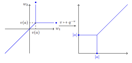
One can sketch a similar picture with \(I=\{a,b\}\), with $\vert a-b\vert_K$ being the distance to the root.

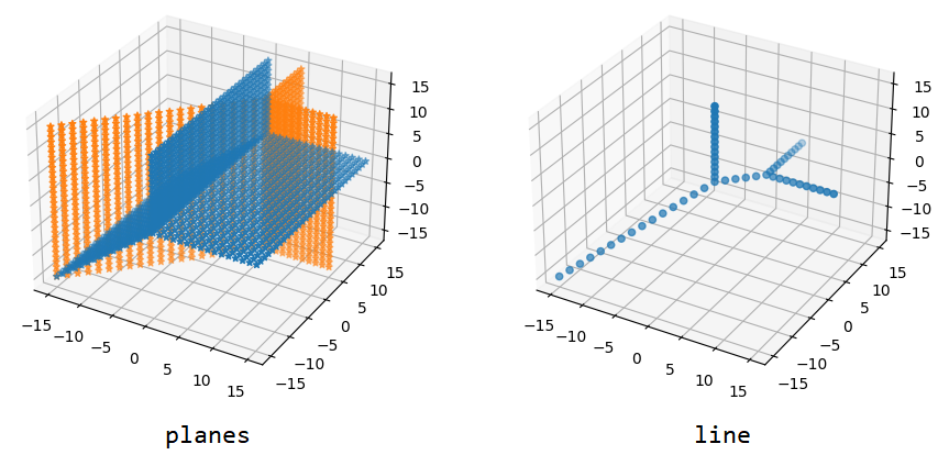
Example 2. Suppose \(I=\{0,a,b\}\), where $\vert b\vert_K>\vert a\vert_K$. Because $X_I\subset\mathbb{A}^3$ is given by equations $T_3=T_1+b$ and $T_2=T_1+a$, we find $\mathrm{trop}(X_I)$ by intersecting tropical varieties $V(\min(w_3,w_1,v(b)))$ and $V(\min(w_2,w_1,v(a)))$. The tropical planes and their intersecting line are plotted below. source code

We observe that, (1) if the line is projected to the $w_1w_2$-plane, then we get back to the picture with \(I=\{0,a\}\), but (2) we also have that $X_I$ (3d picture) is built from \(X_{\{0,a\}}\) by adding a branch to $b$ from (the image of) the ball $B(0,\vert b\vert_K)$.

These observations suggest us the followings.

• Let $J\subset I$ and $\vert I\setminus J\vert=1$. The space $\mathrm{Trop}(X_I)$ is obtained by adding a branch for $a\in I\setminus J$ to a smaller picture $\mathrm{Trop}(X_J)$. If $a_{j_0}\in J$ is such that $\min_{a_j\in J}\vert a-a_j\vert_K=\vert a-a_{j_0}\vert_K$, then the branch is made at the ball norm $B(a_{j_0},\vert a-a_{j_0}\vert_K)$.
• Furthermore, the natural projection $\mathrm{Trop}(X_I)\to\mathrm{Trop}(X_J)$ is obtained by collapsing that branch to the ball norm that had budded the branch.

We thus conclude that, we can sketch $\mathrm{Trop}(X_I)$’s by hand, and even understand the natural projections $\mathrm{Trop}(X_I)\to\mathrm{Trop}(X_J)$ (for $I\supset J$) by hand!

Remark. Other than ‘collapse the branch’ projections, the branching constructions remind us the visualization of the Berkovich line in the previous post. However, although this branching construction is suitable to cover all evaluation and ball norms, it is not very suitable to (1) introduce void intersection norms, and (2) claim density of evaluation norms.

Rather, the picture understanding lures us to the direct limit along the inclusions $\mathrm{Trop}(X_J)\hookrightarrow\mathrm{Trop}(X_I)$ (for $J\subset I$). This gives a different topological space from the inverse limit, $(\mathbb{A}^1_K)^{an}\xrightarrow{\sim}\varprojlim\mathrm{Trop}(X_I)$.

Step 2

Because $\mathbb{A}^1(K)\subset(\mathbb{A}^1_K)^{an}$ is dense, if we do not think it carefully it seems like the equality $\pi_I\left((\mathbb{A}^1_K)^{an}\right)=\overline{\pi_I(\mathbb{A}^1(K))}$ follows for free. But if we set $f=\pi_I\circ ev$ and $A=\mathbb{A}^1(K)$, we are actually claiming $f(\overline{A})=\overline{f(A)}$ here, which is stronger than $f(\overline{A})\subset\overline{f(A)}$, a ‘definition’ of continuity.⁵

Thanks to the following topology fact,

Proposition. If $f\colon X\to Y$ is continuous and proper,^a and $Y$ is locally compact and Hausdorff, then for any $A\subset X$, we have $f(\overline{A})=\overline{f(A)}$.

(Proof) If $y\in\overline{f(A)}$, then there is a compact neighborhood $L$ of $y$ and a net \((f(a_\alpha))_{\alpha\in D}\to y\), with \(a_\alpha\in A\) and \(f(a_\alpha)\in L\). Because $f^{-1}(L)$ is compact, passing to a subnet, we may assume that the net \((a_\alpha)_{\alpha\in D}\) converges to $x\in \overline{A}$. Then \(f(x)=\lim_{\alpha\in D}f(a_\alpha)=y\). $\square$

^{a. The inverse image of any compact set is compact. Equivalently, any net $(x_\alpha)$ in $X$ going to infinity (i.e., escapes any compact set eventually) also has $(f(x_\alpha))$ in $Y$ going to infinity. ↩}

we see that $\pi_I\left((\mathbb{A}^1_K)^{an}\right)=\overline{\pi_I(\mathbb{A}^1(K))}$ is a consequence of the following

Claim. The map $\pi_I\circ ev$ is proper.

(Proof) Denote $x\vee y:=\max(x,y)$, $x\wedge y:=\min(x,y)$, and $\bigwedge_{i\in I}x_i:=\inf_{i\in I}x_i$.

As the map \(ev\colon(\mathbb{A}^1_K)^{an}\hookrightarrow\prod_{a\in K}(-\infty,\infty]\) is a topological embedding, it suffices to see that the set \(ev\left[(\pi_I\circ ev)^{-1}(\mathcal{K})\right]\) is compact for any compact $\mathcal{K}\Subset(-\infty,\infty]^I$.

Observe that

for any $a\in K$, $a_i\in I$, and $M\in\mathbb{R}$. Encoding this set theoretically, we then have the following inclusion:

To conclude that $ev[(\pi_I\circ ev)^{-1}(\mathcal{K})]$ is compact (whenever $\mathcal{K}\subset[M,\infty]^I$ is compact) from this inclusion, we need to know that \(ev\colon(\mathbb{A}^1_K)^{an}\hookrightarrow\prod_{a\in K}(-\infty,\infty]\) is an embedding into a closed subspace. This requires that the map \(\varprojlim\pi_I\colon(\mathbb{A}^1_K)^{an}\to\varprojlim\pi_I((\mathbb{A}^1_K)^{an})\) is surjective, as established in the next section.

$\square$

Step 3

In general, the inverse limit of finite approximations $\pi_I((\mathbb{A}^1_K)^{an})$ is bigger than the original space $(\mathbb{A}^1_K)^{an}$. Thus to have a homoeomorphism, we at least need to know whether the map $\varprojlim\pi_I$ in \eqref{eqn:finite-approximation} is surjective.

The proof below is motivated from (Payne 2009, Proof of Thm. 1.1).

Suppose \((y_I)_{I\subset K}\) is a point in \(\varprojlim\pi_I((\mathbb{A}^1_K)^{an})\). Let $g\colon K[T]\to[0,\infty)$ be a multiplicative function such that $g(a)=\vert a\vert_K$ and $g(T-a)=q^{-y_{{a}}}$, for all $a\in K$. It remains to see if $g$ is a seminorm, i.e., satisfies the triangle inequality \(g(f_1(T)+f_2(T))\leq g(f_1(T))+g(f_2(T))\).

The inequality is trivial if $f_1=0$, $f_2=0$, or $f_1+f_2=0$. So I suppose none of them are the case. Let $I$ be the collection of zeroes of $f_1$, $f_2$, and $f_1+f_2$. Because \(y_I=(y_{\{a\}})_{a\in I}\in\pi_I((\mathbb{A}^1_K)^{an})\) is in the image of the multiplicative seminorms, we have a point \(\vert\cdot\vert_x\in(\mathbb{A}^1_K)^{an}\) such that \(\vert T-a\vert_x=q^{-y_{\{a\}}}=g(T-a)\) holds for all $a\in I$. Because both $\vert\cdot\vert_x$ and $g$ are multiplicative, it follows that \(\vert f_1\vert_x=g(f_1)\), \(\vert f_2\vert_x=g(f_2)\), and \(\vert f_1+f_2\vert_x=g(f_1+f_2)\). The rest follows from the triangle inequality of $\vert\cdot\vert_x$.

This verifies that $g$ is a seminorm on $K[T]$, i.e., \(g\in(\mathbb{A}^1_K)^{an}\). This $g$ has \(\varprojlim\pi_I(g)=(y_I)_{I\subset K}\), as required.

^{5. A quick example of this distinction is $f(x)=\arctan x$, $f\colon\mathbb{R}\to\mathbb{R}$. Indeed, $f(\overline{\mathbb{Q}})=(-\frac{\pi}{2},\frac{\pi}{2})\neq\overline{f(\mathbb{Q})}=[-\frac{\pi}{2},\frac{\pi}{2}]$. ↩}

Appendix: Inverse Limit

Suppose a family \((X_\alpha)_{\alpha\in D}\) of topological spaces are given, indexed by a directed set $D$ (a set with a preorder that admits an upper bound of any two elements). Suppose further that, whenever $\alpha\leq\beta$ in $D$, we have a map \(\varphi_{\alpha\leftarrow\beta}\colon X_\beta\to X_\alpha\). In that case, we define the inverse limit $\varprojlim_{\alpha\in D}X_\alpha$ by the topological space $X$ with the following properties.

• (Natural projections) For each $\alpha\in D$, there is a map $\varphi_\alpha\colon X\to X_\alpha$, such that $\varphi_{\alpha\leftarrow\beta}\circ\varphi_\beta=\varphi_\alpha$ for all $\alpha\leq\beta$ in $D$.
• (Universality) For any space $Y$ with a family of maps $\psi_\alpha\colon Y\to X_\alpha$ such that $\varphi_{\alpha\leftarrow\beta}\circ\psi_\beta=\psi_\alpha$, we have a unique map $f\colon Y\to X$ so that $\psi_\alpha = \varphi_\alpha\circ f$ for all $\alpha\in D$.

The first property indicates that $X$ “stays above all $X_\alpha$’s,” and the second property tells $X$ is the ‘smallest’ among such. The above properties do guarantee uniqueness (up to a homoeomorphism) but do not immediately give the existence of such an object. The existence is established first by constructing the space, e.g.,

A subset $D’\subset D$ is called cofinal if every $\alpha\in D$ has $\beta\in D’$ such that $\alpha\leq\beta$. Then one can show that $\varprojlim_{\beta\in D’}X_\beta\cong\varprojlim_{\alpha\in D}X_\alpha$, applying the universality.

Note for Payne’s Theorem. The directed set in the Payne’s theorem collects all embeddings $i\colon X\to\mathbb{A}^{m(i)}$ of an affine variety $X$ over $K$. We say $i\leq j$ if there is an equivariant morphism $\varphi\colon\mathbb{A}^{m(j)}\to\mathbb{A}^{m(i)}$^a such that $\varphi\circ j=i$.

For $X=\mathbb{A}^1$, an embedding is determined by polynomials $f_1,\ldots,f_m$ by the map $i\colon X\to\mathbb{A}^m$, $T\mapsto (f_1(T),\ldots,f_m(T))$. List all prime factors of $f_i$’s as \((T-a_j)_{j=1}^N\), and let \(\alpha^i_j\) be the multiplicity of $(T-a_j)$ in \(f_i(T)\), and let \(c_i\) be the highest coefficient of \(f_i(T)\). Then one can write \(f_i(T)=c_i\prod_{j=1}^N(T-a_j)^{\alpha^i_j}\).

Define the map $j\colon X\to\mathbb{A}^N$, $T\mapsto(T-a_j)_{j=1}^N$. The map $\varphi\colon\mathbb{A}^N\to\mathbb{A}^m$, $\varphi(S)=(c_1S^{\alpha^1},\ldots,c_mS^{\alpha^m})$ (multiindex notation) is an equivariant map such that $\varphi\circ j=i$. By this, we conclude that $j\geq i$. In other words, the subcollection of linear embeddings of $\mathbb{A}^1$ forms a cofinal family.

Notice that, for linear embeddings $\iota_I\colon\mathbb{A}^1\to\mathbb{A}^I$ and $\iota_J\colon\mathbb{A}^1\to\mathbb{A}^J$, the only way to have $\iota_I\leq\iota_J$ is to have $I\subset J$. Thus we can reduce equivariant preorder to the subset relation.

^{a. That is, there is an algebraic group map $f\colon T^{m(j)}\to T^{m(i)}$ such that $\varphi(a.T)=f(a).\varphi(T)$.↩}

Now suppose a topological space $X$ embeds into a product space $\prod_{\alpha\in\Lambda}X_\alpha$ ($\Lambda$ is just a set). Set $D$ for all finite subsets of $\Lambda$; this forms a directed set by the subset relation. Write $Y_I$ for the image of $\varphi_I\colon X\hookrightarrow\prod_{\alpha\in\Lambda}X_\alpha\twoheadrightarrow\prod_{\alpha\in I}X_\alpha$, and let $Y=\varprojlim_{I\in D}Y_I$ be the inverse limit.

Denoting the natural projection $\pi_{JI}\colon\prod_{\alpha\in I} X_\alpha\twoheadrightarrow\prod_{\alpha\in J} X_\alpha$, we see that whenever $J\subset I$, we have $\varphi_J=\pi_{JI}\varphi_I$. This induces

• a natural map $\varphi\colon X\to Y$.

This map is a topological embedding, but not in general surjective; if $\varphi$ is surjective, then it is automatically a homeomorphism. To see why $\varphi$ is an embedding, note that there is an embedding (defined with the set-theoretic construction) $Y\hookrightarrow\varprojlim_{I\in D}X_I$, where \(X_I=\prod_{\alpha\in I}X_\alpha\) is a subproduct of the product \(\prod_{\alpha\in\Lambda}X_\alpha\), directed with the projections \(\pi_{JI}\colon X_I\to X_J\) for $J\subset I$. Now by checking the universal properties, one has \(\varprojlim_{I\in D}X_I\cong\prod_{\alpha\in\Lambda}X_\alpha\). Stitching all the maps,

we recover the original embedding \(X\hookrightarrow\prod_{\alpha\in\Lambda}X_\alpha\). So the first strand $\varphi\colon X\to Y$ should be an embedding.

Update Log

• 220813: Created
• 220914: Fixed a fatal math mistake