This note is to record some tales that may be adequate while introducing Intermediate Value Theorem (IVT) and Extreme Value Theorem (EVT) for continuous functions. Some ideas behind the proofs, a relation with long division algorithm, etc. are introduced.

Backgrounds

Many calculus texts (Stewart, Thomas, …) introduce the following theorems of continuous functions.

Intermediate Value Theorem. Let $f\colon[a,b]\to\mathbb{R}$ be a continuous function, and let $K\in\mathbb{R}$ be a number between $f(a)$ and $f(b)$. Then there exists $c\in[a,b]$ such that $f(c)=K$.

Extreme Value Theorem. Let $f\colon[a,b]\to\mathbb{R}$ be a continuous function. Then the values $M=\sup_{x\in[a,b]}f(x)$ and $m=\inf_{x\in[a,b]}f(x)$ are attained as function values. That is, there exists $c_1,c_2\in[a,b]$ such that $f(c_1)=M$ and $f(c_2)=m$.

If we understand continuous functions as a ‘function whose graph can be sketched with a continuous path of pencil stroke,’ each theorem has an evident pictorial significance:

• Intermediate value theorem says if we want to connect $(a,f(a))$ and $(b,f(b))$ by a continuous path, one necessarily passes through the horizontal line $y=K$ (provided that $K$ is between $f(a),f(b)$).
• Extreme value theorem says if we want to connect $(a,f(a))$ and $(b,f(b))$ by a continuous path, one cannot go infinitely ‘up,’ nor infinitely ‘down.’

Furthermore, both theorems help us to fill up unconscious gaps that one can make while thinking about continuous or differentiable functions. For instance, in optimization problems of a differentiable function $f\colon[a,b]\to\mathbb{R}$, solving $f’(x)=0$ does help us find global extrema. This is purely because a global extremum exists: solving $f’(x)=0$ can list all local extrema, but checking whether one of them is a global extremum needs a separate argument to guarantee so.

It seems like there is not much further one can say about the theorem, other than speaking of examples and non-examples on the statement of the theorem. But because both theorems are nonconstructive in their statement, one may need to be able to appreciate mathematical abstraction and significance to fully appreciate them.

My understanding is that appreciating mathematical abstraction and significance is sometimes (very often?) a foreign culture for participants in calculus courses. To massage such foreignness, I would note some ‘practical math’ that can explain both theorems: sampling the continuous function.

Sampling

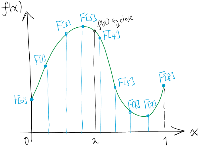
For simplicity, suppose $[a,b]=[0,1]$. (Replace $f(x)$ to $\hat{f}(t)=f\left(a+(b-a)t\right)$ if necessary.) Fix an integer $N>0$ and consider the following data.

This array of $2^N+1$ numbers will be called the $N$-th (binary) sampling of the function $f$. The array elements will be called sampling elements (or samples). It is immediate that elements of the $N$-th sampling are elements of the $(N+1)$-th sampling.

If $f\colon[0,1]\to\mathbb{R}$ is a (uniformly) continuous function, then samplings are good approximations of $f$ in the following sense.

Proposition. Suppose $f\colon[0,1]\to\mathbb{R}$ is (uniformly) continuous. For any $\epsilon>0$, there exists an integer $N>0$ such that for every $x\in[0,1]$, whenever $\vert x-k/2^N\vert \leq 2^{-N}$, we have

\[f(k/2^N)-\epsilon < f(x) < f(k/2^N)+\epsilon.\]

That is, every function value $f(x)$ is less than $\epsilon$ away from some sampling element in some binary sampling.

Sampling a continuous function allows us to (approximately) view a function as a finite array of function values. This viewpoint is used in conventional graphing softwares, where we essentially sample the function, plot the samples, and leave all intermediate parts as “filled up by continuity.” Furthermore, sampling allows us to replace the questions like

• For a number $K$, can we solve $f(x)=K$?
• Does $f$ attain a global maximum or minimum?

to discrete versions like

• For a number $K$, is it appearing as a sampling element? (Or reasonably close to it?)
• Given a sampling, do we have maximal or minimal sampling elements?

Extreme Value Theorem

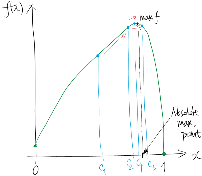
Given the $N$-th binary sampling, it is obvious that we have maximal and minimal sampling elements; just scan through the numbers and record the maximum or minimum. For sake of analysis, name $c_N$ (respectively, $d_N$) for the point $k/2^N$ where $f(k/2^N)$ is maximum (respectively, minimum) among $k=0,1,\ldots,2^N$.

What gets interesting is the phenomena as $N\to\infty$. Because the $(N+1)$-th sampling embraces the $N$-th sampling as a subset, the maximum sampling element gets bigger and the minimum sampling element gets smaller as $N$ increases. That is,

One can raise the following questions.

• Will \(f(c_N)\)’s keep increase and achieve $\sup f([0,1])$ at the limit $N\to\infty$?
• Will \(c_N\)’s head to the global maximum?

We state the dual questions, for sake of completeness:

• Will \(f(d_N)\)’s keep decrease and achieve $\inf f([0,1])$ at the limit $N\to\infty$?
• Will \(d_N\)’s head to the global minimum?

The first question is affirmative as stated, and the second question needs some fix to be affirmative. If we state this formally, we have:

Extreme Value Theorem (with sampling). Let $f,c_N$ be as above.

1. We have \(\left(f(c_N)\right)_{N=1}^\infty\) an increasing sequence, whose limit is same as $\sup_{x\in[0,1]}f(x)$.
2. Any limit point $x$ of the sequence \((c_N)\) is a global maximum.

It turns out that both facts result from continuity, and one can construct examples where the theorem fails without continuity. (Simply let the global maximum be attained at an irrational point whose value cannot be approximated by sampling elements.)

But what is even more interesting is as follows.

• Fact 1. above holds even if the domain is merely a bounded set.
• Fact 2. above holds even if the domain is merely a closed set.

Although standard topology classes view Extreme Value Theorem as a result of compactness, this sampling-based ‘algorithm’ assigns its significance to the closedness and boundedness of the domain. Of course, introducing limit points or closedness are typically out of the scope of regular calculus courses. But it is worth keeping them in mind (as an instructor) because one can attribute topology for examples and non-examples of the EVT.

Sample Lecture Plan

One of the key properties of continuous function defined on a closed and bounded interval, is that one can find an absolute maximum and minimum of the function. To elaborate, we first define some terms.

Definition. Given a (real-valued) function $f(x)$, we say a point $x=x_0$ (in the domain) is an absolute maximum if $f(x_0)\geq f(x)$ holds for all $x$ in the domain; absolute minimum if $f(x_0)\leq f(x)$ holds for all $x$ in the domain.

Then the Extreme Value Theorem is stated as follows.

Extreme Value Theorem. Let $f\colon[a,b]\to\mathbb{R}$ be a continuous function defined on a closed and bounded interval. Then the function $f$ has an absolute maximum and an absolute minimum.

The theorem itself does not tell on how to find absolute maximum or minimum; it only tells there is one. Perhaps one can list all possible candidates (using derivatives) and find one that works the best; but to guarantee that the absolute maximum or minimum is within these candidates, we first need to know that they exist. The theorem is guaranteeing such a fact. Although we will later work on methods using derivatives to find absolute (or local) maxima or minima, it is still interesting to introduce a method - to find absolute maxima or minima - that applies to all continuous functions, differentiable or not. The method is called the sampling method. This is never meant to be an efficient algorithm, but works for any continuous function, differentiable or not - so it can deal with some pathological functions, say nowhere differentiable functions. (See Weierstrass function or Wiener process.)

The idea is this. Given a continuous function $f\colon[0,1]\to\mathbb{R}$, suppose we record the function as a list $F[k]:=f(k/2^N)$. (Or more generally, $F[k]=f(a+(b-a)k/2^N)$ if f is defined on $[a,b]$.) This array $F[0],F[1],\ldots,F[2^N]$ of length $2^N+1$ is a reasonable approximate representation of the function. For instance, for any $\epsilon>0$ of your choice, one can set $N$ large enough, so that plotting $(k/2^N,F[k])$ and connecting them through lines gives an approximate graph of $f(x)$ with the error kept $<\epsilon$ (justifying it requires some advanced notion of continuity, however).

We call the array $F[0],F[1],\ldots,F[2^N]$ the $N$-th binary sampling of the function $f(x)$, and call elements of this array as sampling elements. This may be seen as a way to record our function $f(x)$ within a computer.

If we have a list of numbers, we can easily find its maximum within that list. Furthermore, that maximum in the sampling well approximates an absolute maximum, too. By this note, one can propose the following 'algorithm' to find an absolute maximum.

• Make the $N$-th binary sampling, with $N$ large.
• Find a maximum sampling element; call it \(F[k_N]=f(c_N)\) (i.e., \(c_N=k_N/2^N\)).
• Increase $N$ over and over. The maximum sample element \(F[k_N]\) then converges to the absolute maximum value of $f$, and points \(c_N\) on the domain approximate an absolute maximum point of $f$.

This method of finding an absolute maximum of a continuous function is based on a fairly straightforward algorithm of finding the maximum of a finite list of numbers. However, it has clear drawbacks: no one can guarantee that the maximum sampling element of the $(N+1)$-th binary sampling is found somewhere near that of the $N$-th binary sampling. (See Remark below.) Because step $N$ does not (necessarily) help for step $(N+1)$, one needs to look up the entire sampling every time when one increases $N$. This is definitely a waste of computational resources!

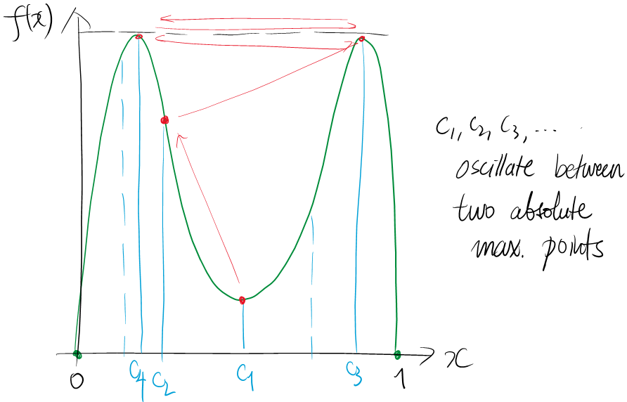
Remark. One warning about the maximum point $c_N$ within the sampling is that, the points $$c_1,c_2,\ldots$$ may oscillate between two points.

This is typically the case when there is more than one absolute maximum point. In that case, the maximum sampling element $$F[k_N]=f(c_N)$$ may be found at multiple places, causing the oscillation of concern. However, choosing one 'place' (or 'region') of oscillation suffices to find an absolute maximum.

Remark. However, in most of practical calculus examples we only have a few spots that admits maximum sampling element. But these spots may not be seen from samplings alone. Rather, we spot them using methods of derivatives. Perhaps they serve some good ways to get rid of the inefficiency of tracing all samples!

There are a few cases where the algorithm does not work as intuitively understood. This is often caused by dropping continuity or dropping assumptions about the domain - closed and bounded.

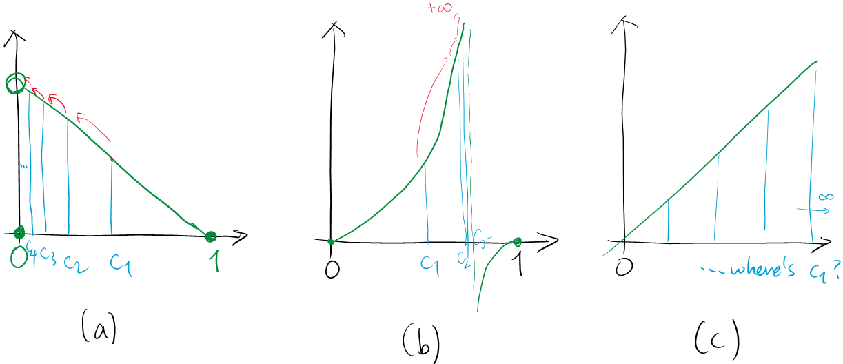
1. When the maximum sampling elements suggest an 'absolute maximum' that is not an absolute maximum. See (a) below.
2. When we keep increase $f(c_N)$'s and reach to infinities. See (b) below.
3. When the domain is unbounded so that $c_N$'s are not even defined. See (c) below.

We should thus understand that the assumptions that (1) the function has domain as a closed interval, and (2) the function is continuous, as assumptions that are designed for the algorithm to work properly. It is left as an exercise to think of how absolute minima is found by the sampling method.

Acknowledgement

This idea of sampling a continuous function and application to the Extreme Value Theorem came from personal communication with Junekey Jeon.

Intermediate Value Theorem

With the method of sampling, the intermediate value theorem is ought to be ‘proven’ by the bisection method. Here we keep our assumption $[a,b]=[0,1]$ here; we further assume $K=0$ and $f(0)<0<f(1)$. (Replace $f(x)\leftarrow K-f(x)$ or $f(x)\leftarrow f(x)-K$ if necessary.)

Standard proof of the Intermediate Value Theorem starts by taking the following supremum.

Then one challenges to show that $f(c)=0$ from this setup.

This proof has a straightforward translation in terms of the sampling method. Simply take the nonpositive sampling element $f(k/2^N)$ where $k=0,1,\ldots,2^N$ is set as big as possible. The sequence $c_N=k/2^N$ obtained is an increasing sequence whose limit is a zero of $f(x)$. (More precisely, $c_N\to c$.)

However, proving that $c=\lim c_N$ is a zero of $f(x)$ requires some smart use of the squeeze method, as sketched below.

Suppose $f(c)\neq 0$. Set $\epsilon=\frac12\vert f(c)\vert$ and choose $N$ according to a Proposition above. By the definition of $c_N$, we have $c_N=\lfloor 2^Nc\rfloor/2^N$ and $f(c_N)\leq 0<f(c_N+2^{-N})$. If $f(c)<0$, then $0<f(c_N+2^{-N})<f(c)+\epsilon=\frac12 f(c)<0$ gives a contradiction. If $f(c)>0$, then $0\geq f(c_N)>f(c)-\epsilon=\frac12f(c)>0$ gives a contradiction.

Perhaps building up this proof can be an interesting exercise for an analysis course. But it seems like this proof is out of the scope of a regular calculus course. Nonetheless, stating that the sampling method still gives an idea to prove IVT, seems worth introducing.

Bisection method

One consequence of the Intermediate Value Theorem is the bisection method, a numerical algorithm to find a zero of a continuous function. The method is aimed to ‘squeeze’ the possible range $[a_N,b_N]$ of finding a zero. To formally write this as a form of an algorithm, we say:

1. Make sure that $f$ is continuous and $f(0)<0<f(1)$.
2. Set $(a_1,b_1)=(0,1)$.
3. For each $N=1,2,3,\cdots$, define $(a_{N+1},b_{N+1})$ by the following case-by-case basis.
   1. If $f(\frac12(a_N+b_N))=0$, return $c=\frac12(a_N+b_N)$ and terminate.
   2. If $f(\frac12(a_N+b_N))<0$, set $(a_{N+1},b_{N+1})=(\frac12(a_N+b_N),b_N)$.
   3. If $f(\frac12(a_N+b_N))>0$, set $(a_{N+1},b_{N+1})=(a_N,\frac12(a_N+b_N))$.
4. If the above procedure does not terminate, set $c=\lim_{N\to\infty}c_N$.

One can show that the pair $(a_{N+1},b_{N+1})$ appears as consecutive elements in the list $0/2^N,1/2^N,\ldots,2^N/2^N$. Thus the method is somewhat relevant to the sampling method. Furthermore, the method gives proof of the Intermediate Value Theorem in the following sense.

Intermediate Value Theorem (by bisection method). Let $c$ be the number found above. Then we have $f(c)=0$.

However, the proof is again requiring some analysis. One needs (i) the notion of the Cauchy sequence to ensure that the limit $c=\lim c_N$ exists, and (ii) some smart use of the uniform continuity to apply the ‘squeeze method’ and obtain $f(c)=0$.

Decasection method

Now the bisection method is most likely to be a foreign method for average students. One way to convey the method as something familiar is to upgrade this to a ‘deca-section method,’ meaning that we update $(a_N,b_N)$ by

• $a_{N+1}=a_N+q\cdot 10^{-N}$ and $b_{N+1}=a_N+(q+1)\cdot 10^{-N}$, where $q=0,1,\ldots,9$ is a number such that $f(a_N+q\cdot 10^{-N})\leq 0\leq f(a_N+(q+1)\cdot 10^{-N})$.

(This method can be conveyed better if one has a picture that subdivides $[a_N,b_N]$ into 10 equal pieces and choose one that passes through a zero of $f(x)$.)

This can be still new for the version stated above, but if one thinks of a division problem, the matter will get more familiar. Say, consider $13\div 9$. Setting $f(x)=9x-13$ one has $f(0)=-13<0<f(10)=77$, and updates $(a_1,b_1)=(0,10)$ as follows.

• Since $f(1)=-4<0<f(2)=5$, we update $(a_2,b_2)=(1,2)$;
• since $f(1.4)=-0.4<0<f(1.5)=0.5$, we update $(a_3,b_3)=(1.4,1.5)$;
• since $f(1.44)=-0.04<0<f(1.45)=0.05$, we update $(a_4,b_4)=(1.44,1.45)$,

etc. It is now evident that we are essentially running the long division algorithm, but stated in the calculus language. Even, this will be a moment when students see that the long division algorithm (that they may be encountered around a decade ago) is mathematically justified. If possible, then one can leverage this to appreciate the beauty of mathematical rigor or abstractions.

This decasection method not only justifies the traditional (numerical) division algorithm but also applies to finding zeroes of polynomials numerically. For instance, one can ask to compute $\sqrt{0.5}$ by applying the decasection method to $f(x)=x^2-0.5$. Computations are typically painful in this direction, but one can obtain $\sqrt{0.5}=0.707\ldots$, a fairly good estimate, just before seeing some heavy numbers.

Update Log

• 221127: Created
• 221212: Hashing -> Sampling, and fixing some conceptual remarks that sounds misleading (after some discussion with Junekey Jeon
• 230413: Some typo fixes