A summary of the basics of the Ruelle transfer operator, along with some notes about how potentials work in the context of Szilard’s engine.

Definitions

Most of the definitions below are from Ruelle 1992.

Transfer Operator

Let $(X,d)$ be a compact metric space and $f\colon X\to X$ be a continuous map, which we call $(X,f)$ a topological dynamical system. We call a function $A\colon X\to\mathbb{R}$ a potential. Then we define an operator $\mathcal{L}=\mathcal{L}_{f,A}$ as

for $\omega$ in a suitable function space on $X$. This operator $\mathcal{L}$ is called the transfer operator or the Ruelle(-Perron-Frobenius) operator.

If the domain of $\mathcal{L}$ contains continuous functions, then we think of its adjoint operator $\mathcal{L}^\ast$ acting on measures as well. If $f$ is differentiable, then we can set $A=-\log\vert J_f\vert$, where $J_f$ is the Jacobian of $f$, to get $\mathcal{L}^\ast=f_\ast$.

Expansive, Specifications

We say a topological dynamical system $(X,f)$ is expansive and has specifications if it satisfies the following:

• We say a system is expansive with expansive constant $C>0$ if $d(f^ix,f^iy)<C$ for all $i=0,1,2,\ldots$ implies $x=y$.
• We say a system has specifications if for every $\epsilon>0$ there is an integer $p=p(\epsilon)>0$ such that, given $\ell$ points $x_1,\ldots,x_\ell\in X$ and integers $n_1,\ldots,n_\ell>0$, $p_1,\ldots,p_{\ell-1}\geq p$, there exists $z\in X$ such that

for $i=0,\ldots,n_j-1$ and $j=1,\ldots,\ell$, where $m(j)=n_1+p_1+\cdots+n_j+p_j$.

Expansive means if two trajectories stay within a certain distance, then they must be the same. Having specifications means the list of points

can be approximated by an orbit $(f^jz)_{j\geq 0}$ as long as the empty buffers are long enough.

Both properties reminisce some properties of Anosov diffeomorphisms.

Bowen potential

This concept is mentioned by Ruelle but not named. The term ‘Bowen property’ is taken from other works, such as Call 2020 (see Definition 2.18).

Given a topological dynamical system $(X,f)$ and a potential $A\colon X\to\mathbb{R}$, we say $A$ has the Bowen property at scale $\epsilon>0$ if

If $(X,f)$ is expansive, then we say a potential $A$ has the Bowen property if it has the Bowen property at the expansive constant.

Gibbs measure

Let $U\subset X$ be a compact subset and $\varphi\colon U\to\varphi(U)\subset X$ be a homeomorphism onto its image. We say a pair $(U,\varphi)$ is a conjugating homeomorphism if for each $x\in U$ we have $\lim_{k\to\infty}d(f^kx,f^k\varphi x)=0$.

Let $A$ be a potential that is Bowen. We say a probability measure $\mu\in\mathcal{M}^1(X)$ is a Gibbs state for $A$ if for any conjugating homeomorphism $(U,\varphi)$, we have

That is if we say

then the criterion \eqref{eqn:gibbs-measure} is formally rewritten

although the convergence of \(\mathcal{E}\{A\}\) is not guaranteed so the expression \eqref{eqn:gibbs-measure-formal} is just formal.

Topological Pressure

Let $(X,f)$ be a topological dynamical system. Let $\mu$ be an invariant probability Radon measure. Its measure-theoretic entropy or Kolmogorov-Sinai entropy is denoted $h_\mu(f)$; for its definition, refer to Scholarpedia, Wikipedia, or standard textbooks like Walter 1982. Recall also that $\mu\mapsto h_\mu(f)$ is affine (i.e., $h_{(1-p)\mu+p\nu}(f)=(1-p)h_\mu(f)+ph_\nu(f)$); see Walter 1982, Theorem 8.1.

Denote $\mathcal{M}(X)^f$ for the space of invariant probability Radon measures on $X$. This forms a convex set, and the negentropy map $\mu\mapsto -h_\mu(f)$ is a convex function on it. Therefore one can think of its convex conjugate

which is called the topological pressure of $(X,f,\mu)$ by the potential $\phi$. We say $\mu\in\mathcal{M}(X)^f$ an equilibrium state for $A$ if the supermum is attained at $\mu$.

It obviously follows that $P(\phi)$ is convex in $\phi$, and $P(0)=h_{\mathrm{top}}(f)$ is the topological entropy.

By the natural duality of measures and continuous functions, $\phi$ is morally a continuous function. But I will also abuse the notations and think of $P(\phi)$ for measurable functions, whenever defined. For instance, Bowen potentials well-define the pressure.

Walter’s Theorem

Walter 1975, Theorem 4.1 proves the variational principle for topological pressures defined with separating sets. This compares the topological pressures, defined with the measure-theoretic definition \eqref{eqn:measure-theoretic-pressure} and the topological definition \eqref{eqn:topology-pressure} stated below.

Given a topological dynamical system $(X,f)$, we say a finite set $E\subset X$ is $(\epsilon,n)$-separated if any distinct $x,y\in E$ has $d(f^ix,f^iy)>\epsilon$ for all $i=0,1,\ldots,n-1$. Then we define

and

This reminds us of the definition of topological entropy using separated sets, especially when $\phi\equiv 0$. Walter’s theorem states that definitions \eqref{eqn:measure-theoretic-pressure} and \eqref{eqn:topology-pressure} coincide.

Ruelle-Perron-Frobenius Theorem

Ruelle then proved the following.

Theorem (Ruelle 1992). Let $(X,f)$ be a topological dynamical system that is expansive and has specifications. Given a Borel function $A$ that has the Bowen property, the following hold.

1. There is a unique equilibrium state $\rho$ for $A$.
2. There is a unique Gibbs state $\mu$ for $A$, which satisfies the following eigen-measure property:

\(\mathcal{L}^\ast\mu = e^{P(A)}\mu.\)

1. There is a unique $\Phi\in L^1(\mu)$ such that $\rho=\Phi\mu$, and $\Phi$ is (up to a constant) the only eigenfunction of $\mathcal{L}$ acting on $L^1(\mu)$, which is positive and $\log\Phi\in L^\infty(\mu)$:

\[\mathcal{L}\Phi = e^{P(A)}\Phi.\]

1. Let $\Psi\in L^p(\mu)$, $1\leq p<\infty$. Then we have, in $L^p(\mu)$,

\[\lim_{n\to\infty}e^{-nP(A)}\mathcal{L}^n\left(\Psi-\Phi\cdot\int_X\Psi\,d\mu\right)=0.\]

The importance of the result cannot be overemphasized, so I will point out only a piece of it: topological pressure is seen as the logarithm of the ‘Perron-Frobenius eigenvalue’ of the transfer operator.

Transfer Operators on Shift Spaces

To study the definitions above further, we study what happens to the definitions for the space \(X=\{0,1\}^\mathbb{N}\) of full shifts (here, our natural number set \(\mathbb{N}=\mathbb{Z}_{>0}\) consists of positive integers). We denote an element \(\left(x_i\right)_{i=1}^\infty\in X\) as digits after a point, \(.x_1x_2x_3\cdots\).

Perhaps we can append some alphabets in front of $x\in X$. Such elements will be denoted $.0x$, $.1011x$, etc.

The natural dynamics that the shift X carries is the shift map,

To describe the topology, we denote the cylinder set as $C(.0)$, $C(.0\mathrm{x}1)$, etc. That is, given a finite string in 0, 1, and x, we collect elements of the shift X that follows the pattern (where x is interpreted as ‘free’). So for instance,

We fix any number $0<\theta<1$ and define the metric on X by

By this metric, the shift system $(X,\sigma)$ is expansive (with constant $\theta$) and has specifications.

Zero potential

Denote \(\mathcal{L}_0\) for the transfer operator with the zero potential $A\equiv 0$. That is, \(\mathcal{L}_0\omega(x)=\sum_{y\colon\sigma(y)=x}\omega(y)=\omega(.0x)+\omega(.1x)\). A picture for this action may be sketched as follows.

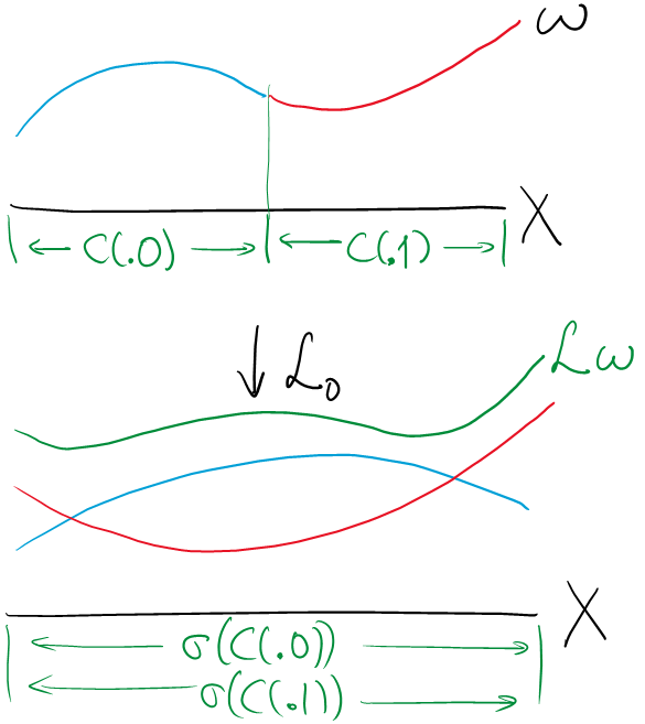
That is, we think of restrictions $\omega\vert C(.0)$ and $\omega\vert C(.1)$, “stretch the domains” (by the shift map $\sigma$) for each, and add them up to find \(\mathcal{L}_0\omega\).

A handy way to discover this is to try evaluating $\mathcal{L}_0\omega$ for some 'sample continuous functions' $\omega=\mathbf{1}_{C(.0)},\mathbf{1}_{C(.01)}-\mathbf{1}_{C(.00)}$, etc. Such combinations of indicator functions are easy to sketch and easy to trace their contributions, thus the pictorial interpretation above.

If we think $\omega$ as a mass distribution over $X$, then \(\mathcal{L}_0\omega\) is the new mass distribution obtained by acting the shift $\sigma$ to the space $X$. As we do not normalize the mass after the procedure, it is easy to guess that overall mass doubles after each step, and there seems no additional ‘concentration of mass’ that exhibits an increase of mass of more than two times. Thus we guess that the Perron-Frobenius eigenvalue is 2. Indeed this matches with \(h_{\mathrm{top}}(X,\sigma)=\log 2\).

Bernoulli Potential

Next, we think of the potential \(A=\beta\mathbf{1}_{C(.0)}\), where $\beta\in\mathbb{R}$ is a real parameter. That is, we have $A(x)=\beta$ if $x\in C(.0)$, and $A(x)=0$ otherwise. Call \(\mathcal{L}_\beta\) for the corresponding transfer operator.

In that case \(\mathcal{L}_\beta\omega(x)=e^\beta\omega(.0x)+\omega(.1x)\), so it does a similar job as the zero potential cases, except that it emphasizes (or dismisses, if $\beta<0$) mass located at the cylinder $C(.0)$. The process multiplies the mass by $(e^\beta+1)$, so just as the \(\mathcal{L}_0\) case, we guess the Perron-Frobenius eigenvalue of \(\mathcal{L}_\beta\) as that multiple.

Indeed, the sequence \((e^\beta+1)^{-n}\mathcal{L}_\beta^n\omega\), where $\omega$ is the indicator function of a cylinder set of $X$, converges to the constant function \(\int_X\omega\, d\mu_\beta\), where $\mu_\beta$ is the Bernoulli measure defined as follows.

For any cylinder $C(.s)$, let $\vert s\vert_0,\vert s\vert_1$ be the number of 0’s and 1’s appearing in $s$, respectively. Let $p=(1+e^{-\beta})^{-1}$. Then we define

\[\mu_\beta(C(.s))=\binom{\vert s\vert_0+\vert s\vert_1}{\vert s\vert_0}p^{\vert s\vert_0}\left(1-p\right)^{\vert s\vert_1}.\]

This verifies that \(\mathcal{L}_\beta\) has the Perron-Frobenius eigenvalue $(e^\beta+1)$, the eigenfunction 1, and the eigenmeasure (which is a Gibbs measure; consider the homeomorphism fixing a digit $C(.0)\to C(.1)$) \(\mu_\beta\) which is the Bernoulli measure above. The eigenmeausre is also the equilibrium measure for the potential \(A=\beta\mathbf{1}_{C(.0)}\), and thus the pressure is

where $p=(1+e^{-\beta})^{-1}$.

Szilard’s Engine, Boltzmann Distribution

The Engine

Here is an attempt to relate the topological pressure with Szilard’s engine. (Figure from Leff & Rex 2002)

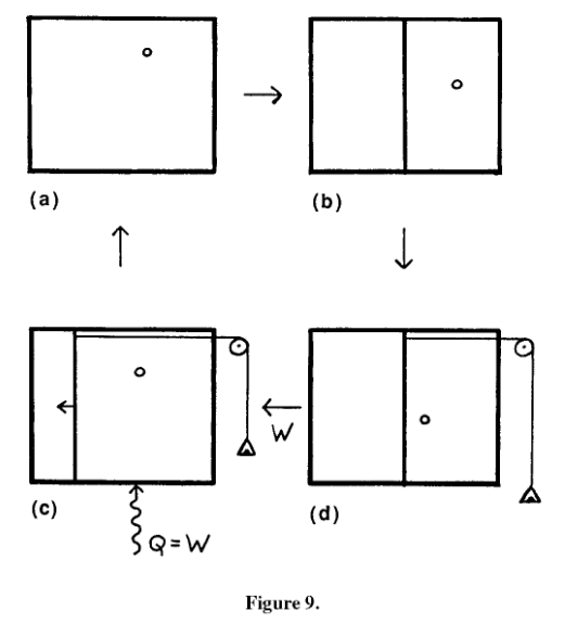
Szilard’s engine is an ideal model of an information engine, that consists of a chamber that has one particle of an ideal gas (fig. (a)); thus the state equation $\beta VP=1$, where $\beta=1/(k_BT)$ is the inverse temperature. The cyclic operation of the engine is described as follows.

The chamber of the engine is first partitioned into two (equal) parts, and one observes at which partition the particle land (fig. (b)). Based on that information, one turns the partition into a piston (fig. (c)). One then receives heat from the heat bath to run the piston (fig. (d)). By this, we come back to the initial stage (fig. (a)).

Hence during the cycle, we see that the machine turns heat energy $Q$ to some work $W$ for free, modulo any changes made during the observation. But one also needs to be clear that in fig. (b), we have changed from a state with two possibilities ($S=k_B\log 2$) to a state with one possibility ($S=0$). By this, we have discovered some entropy change that was not found when we only traced thermodynamical works (cf. a video lecture, in Japanese), which compensates the apparent paradoxical entropy reduction.

Variant 1

Consider a modification of Szilard’s engine that partitions the chamber unevenly, say $p:(1-p)$ in volume. But regardless of which partition the particle land, we can estimate the work done by the particle during the isothermal process:

Now we estimate the work $W$ case-by-case.

• If the particle is observed in the left partition, then the amount of work exerted is

• If the particle is observed in the right partition, then the amount of work exerted is

Averaging the two, we have

and thus

is recovering the binary Shannon entropy.

Variant 2

Suppose we are building our chamber with a flexible material, so that the chamber may expand one of its partitions to reach the equilibrium. (We initially partition the chamber evenly in volume.)

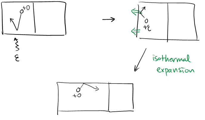
To elaborate, we run the engine as follows. If the particle exists at the left side, add some energy $\epsilon$ to the particle. Using that energy, let the particle isothermally expand. (If the particle exists at the right side, do not add energy, but expand the left chamber \(V_f=e^{\beta\epsilon}V_i\) anyways.)

To estimate the final volume after the expansion $V_i\to V_f$, we think that the energy $\epsilon$ received is completely turned into the work, thus

Hence

By this, we reduce to the uneven volume case, with the volume ratio $e^{\beta\epsilon}:1$. (Observe that the expression reminds us of the Boltzmann distribution, modulo some sign conventions.)

Furthermore, running the remaining steps of the engine we see that the total amount of work done is estimated as follows.

• If the particle exists at the left partition, then

• If the particle exists at the right partition, then

So $\langle W\rangle=\beta^{-1}\log(1+e^{\beta\epsilon})$ and $S=\log(1+e^{\beta\epsilon})$ follows.

If we understand that this $\epsilon$ is taking the role of potential \(\beta\epsilon\mathbf{1}_{C(.0)}\) in the transfer operator over a symbolic system, the entropy computed above is precisely the topological pressure \(P(\beta\epsilon\mathbf{1}_{C(.0)})=\log(1+e^{\beta\epsilon})\) that we have found in \eqref{eqn:pressure-logZ}.

Update Log

• 230111: Created
• 230116: Fixed a misleading description on Variant 2/Szilard’s engine
• 230128: Title changed: there’s no Landauer Principle discussed!